Should meta-scientists hold themselves to higher standards?

This blogpost was written by Michèle Nuijten. Michèle is an assistant professor of our research group who currently studies reproducibility and replicability in psychology. She is also the developer of the tool “statcheck”. This tool automatically checks whether reported statistical results are internally consistent.

As a meta-scientist, I research research itself. I systematically examine the scientific literature to identify problems and apply the scientific method to design and test solutions. Inherent to meta-science is that it can also include critique of other people’s research and advice on how to improve.

But what if meta-scientists don’t always follow the very best practices they promote?

This question came up recently at an event where a high-profile meta-scientific paper was retracted due to misrepresentations of what had and hadn’t been preregistered. The backlash on social media included concerns that the authors had lost (at least some) credibility as advocates of responsible and transparent research.

That reaction stuck with me because it seemed to suggest that, for a meta-scientist to be credible and for their advice to be taken seriously, their own work must be flawless.

So I began to wonder: Should meta-scientists hold themselves to higher standards to maintain credibility? Should I? And how would it affect my own credibility as a meta-researcher if I dropped the ball somewhere along the way?

Dropping the ball

And I definitely did drop the ball. More than once.

For example, I discovered that my dissertation contained statistical reporting errors. The same dissertation in which I studied statistical reporting errors. And for which I developed statcheck, a tool I specifically designed to detect and prevent them.

In that same dissertation, I also examined bias in effect size estimates and advocated for preregistration: publishing a research plan before data collection to reduce analytical flexibility. But, as one of my opponents subtly pointed out during my defense, I hadn’t preregistered that study myself.

Criticizing the field for its high prevalence of statistical errors while making those same errors, or failing to preregister a study that promotes preregistration; what does that say about the validity of my recommendations? And what does it mean for my credibility as a meta-scientist?

Practice what you preach

Technically, you could make strong claims about the benefits of, say, data sharing without ever having shared a single data point yourself, but it’s not a great look.

To some extent, if you want your advice to be taken seriously, you need to practice what you preach. If you keep insisting that everyone should share their raw data, your credibility takes a hit if you never do it yourself. If you argue that all studies should have high statistical power, you’re probably less convincing if your own sample sizes are consistently tiny. And if you’re a vocal advocate for preregistration, it helps to have preregistered at least one of your own studies—if only to truly understand what you’re talking about.

Following your own advice doesn’t just strengthen your credibility; it also gives you firsthand experience with the challenges that can arise in practice. What looks great on paper isn’t always easy to implement. More importantly, by leading by example, you can show others what these practices look like in action and inspire them to follow suit. In this spirit, striving for the highest standards—whether through a flawless preregistration or a meticulously documented open dataset—makes perfect sense.

What is “perfect science”?

While I believe it’s important for meta-scientists to make a genuine effort to implement the changes they advocate, I don’t think it’s necessary—or even possible—to maintain a perfect track record.

One challenge is that best practices evolve over time. Early preregistrations, for example, seem rudimentary compared to today’s standards. What once qualified as “data sharing” may no longer meet current expectations. These shifts reflect a growing understanding of these practices: how they work in practice, their intended and unintended effects, when they are effective, and in some cases, whether they should be abandoned altogether. And both standards and practices are still evolving

Another issue is that not all best practices are feasible for every project. Some conflict with each other (e.g., data sharing vs. privacy concerns), while others may be ethically or practically impossible in certain contexts (e.g., large sample sizes in rare populations). I’ve advocated for a wide range of best practices: open data and materials, preregistration, Bayesian statistics, using statcheck to detect errors, high statistical power, multi-lab collaborations, verification of claims through reanalysis and replication, and more. While I’ve applied all of these practices in at least some of my work, I haven’t (and often couldn’t) apply them all at once. And that’s just the best practices I’ve personally written about; the broader literature contains many more good recommendations.

Credibility of claims, not people

So what does it mean for the credibility of meta-scientists if their own projects can’t even adhere to all best practices? In my view, that’s not the right question to ask. In science, what matters most is not the credibility of a person, but the credibility of a claim. If a claim—whether in applied science or meta-science—is built on shaky evidence, it should carry less weight. The key is to evaluate which best practices are essential for assessing the trustworthiness of a claim and which are less relevant.

For example, the statistical reporting error in my dissertation appeared in a secondary test, buried in a footnote, and had no impact on the main findings. Missing it was an unfortunate oversight, but it didn’t weaken my core claim that a large share of published papers contain reporting errors. On the other hand, one could argue that the claims from my unregistered study should be interpreted with more caution than if it had been preregistered.

Shared standards for good science

At its core, meta-science is simply science, just like applied research. The fundamental principles are the same; the main difference is that our "participants" are often research articles, and our recommendations aim not at populations of patients, adolescents, or consumers, but at the scientific process itself.

With that in mind, both meta-researchers and applied researchers should strive to follow best practices as they currently stand and as they are feasible for their projects. But perfection isn’t the goal. What matters most is transparency: acknowledging when best practices weren’t followed, explaining why, and adjusting how claims are interpreted accordingly. After all, the credibility of a claim should rest on the strength of its evidence, not on whether the person making it has a spotless record.

Science is always evolving, and so are its standards. What matters is not stubbornly trying to check all the boxes of an ever-changing checklist, but a commitment to honesty, critical reflection, and continuous improvement. The best way to build trust in meta-science—or any science—is not to appear flawless, but to openly engage with the challenges, trade-offs, and limitations of our own work. Good science isn’t about being perfect, it’s about being transparent, adaptable, and striving to do better.

Low(er) precision of estimators of selection models: intuition and a preliminary analysis

This blogpost was written by Marcel van Assen. Marcel is a professor of our research group that focuses his research on statistical methods to combine studies, publication bias, questionable research practices, fraud, reproducibility, improving pre-registration & registered reports.

Estimates of random-effects meta-analysis are negatively affected by publication bias, generally leading to overestimation of effect size. Selection models address publication bias and can yield unbiased estimates of effects, but the precision of their estimates is lower than of random-effects meta-analysis. Why and how much precision is lowered has been unclear, and I here provide an intuition and analysis to preliminarily answer these questions. If you are not interested in the details of the analysis, please go directly to the conclusions below.

1.      Accurately estimating effect size with selection models in the context of publication bias

Meta-analysis is used to statistically synthesize information of different studies on the same effect. Each of these studies yields one or more effect sizes, and random-effects meta-analysis combines these effect sizes into one estimate of the average true effect size and an estimate of the variance or heterogeneity of the effect size.

A well-known and serious problem of both the scientific literature and meta-analyses is publication bias. Typically, publication bias amounts to the overrepresentation of statistically significant findings in the literature, or alternatively, the underrepresentation of nonsignificant findings. Because of publication bias meta-analyses generally overestimate the true effect size, and in case of a true zero effect size publication bias likely results in a false positive. Both these consequences are undesirable; we need an accurate estimate of the effectives of an intervention for adequate cost-benefit analyses, and implementing interventions that do not work is very harmful.

One solution of the problem is applying meta-analysis using models that account for the possible effects of publication bias. For example, selection models (e.g., Hedges and Vevea, 2005), including p-uniform* (van Aert & van Assen, 2025). Characteristic of these models is that they categorize effect sizes into at least two different intervals, and that estimation occurs by treating both intervals independently. In the most parsimonious variant of these models, two intervals of effect sizes are distinguished, for instance “effect sizes statistically significant at p < .025, right-tailed” and “other effect sizes”. The critical assumption in all these models is then that the probability of publication of effect sizes within one interval is constant but may differ across different intervals. Indeed, if this assumption holds, and all intervals contain at least some effect sizes, and there is publication bias, selection models and p-uniform* accurately estimate average effect size as well as heterogeneity of effect size (e.g., Hedges & Vevea, 2005; van Aert & van Assen, 2025). Problem solved?

2.      Accurate estimation with selection models comes at a prize: less precision

The price that we pay for accurate estimation with selection models is lower precision of the estimates. Consider the following two examples to consider if we are willing to pay this price. The field of both examples is plagued with publication bias. Hence it can be expected that random-effects meta-analysis overestimates effect size,

In example A the random effects meta-analysis yields an estimated Hedges’ g = 0.7 with SE = 0.1, whereas a selection model yields an estimate equal to 0.6 with SE = 0.2.  Both models strongly suggest that the true effect is positive, although the selection model’s estimate is somewhat lower and considerably less precise.

In example B we obtain Hedges’ g = 0.25 with SE = 0.1 using random-effects meta-analysis and with a selection model we obtain estimate -0.12 with SE = 0.3. Here, random-effect meta-analysis suggests a small and positive true non-zero effect size (z = 2.5, p = .012), whereas the selection model doesn’t lead to a rejection of the null-hypothesis.

The performance of estimators is evaluated using different criteria. One criterion is bias. Concerning bias, selection models outperform random-effects meta-analysis. But as we also prefer precision, we may also use another criterion that combines bias and precision. A criterion that does that is the mean squared error (MSE)

with X being the estimator of parameter µ, and bias equal to (E(X) - µ)^2) .

Let’s apply the MSE to both our examples. For example A, assume that  = .6 and that random-effects meta-analysis overestimates  with 0.1 because of publication bias. Then, MSE of random-effects meta-analysis equals .1 ² + .1 ² = .02, and MSE of the unbiased selection model equals .2 ² + 0 ² = .04, with random-effects meta-analysis being the “winner” with the lowest value of MSE. Concerning example B, assume that  = .2 and the bias equals .2. Then, MSE = .1 ² + .2 ² = .05 for the regular meta-analysis, whereas it equals .3 ² + 0 ² = .09 for the selection model, with again random-effects meta-analysis being the “winner”.

I, however, want to argue that the MSE is not a good criterion to evaluate the performance of estimators of meta-analytic effect size in the context of publication bias. Where it is relatively inconsequential to pick one estimator over the other in example A as both point at a positive effect of considerable size, it is surely consequential in cases like situation B. If  = 0, random-effects meta-analysis overestimates effect size with type I error rates (another relevant performance criterion) close to 1, rather than α, in case of publication bias (e.g., Carter et al., 2019); it provides a precise but very wrong estimate, leading to harmful conclusions about the effectiveness of interventions. Thus, the precision of estimators is important, but its accuracy is sometimes (much) more important. Perhaps we should use another performance criterion MSEMA for effect size estimators in meta-analysis, such as

with a and b being positive constants. Parameter a signifies the extent to which precision is taken into account in the calculation of MSE anyway, whereas b signifies how much of precision is taken into account depending on true effect size. For a = 1 and b = 0, MSE = MS^EMA.  Consider MS^EMA with a = 0 and b = 4. Then, for  = .5 it holds that MSEMA = MSE, but precision gets less emphasis relative to accuracy for  < .5, with only accuracy being relevant for  = 0. For the latter MS^EMA, the random-effects estimator is preferred in Example 1 (1.44 × 0.1² + 0.1² = 0.0244 versus 1.44 × 0.2² = 0.0576), but the selection model estimator is preferred in Example 2 (0 × 0.2² + 0.2² = 0.04 versus 0 × 0.3² + 0² = 0). I argue that more research is needed in developing sensible alternatives to MSE in the context of meta-analysis with publication bias. Estimators belonging to class MSEMA may be a start in that direction.

3.      Why the selection model’s effect size estimate is less precise:  an intuitive explanation

To my knowledge, neither an intuition has been provided nor an examination has been conducted on the reasons for the lower precision of the selection model’s estimate. In this section I hope to provide some intuition, in the next section the results of a preliminary analysis.

Consider a random draw of four observations from a normal distribution with mean 0 and standard deviation 1:

set.seed
help <- rnorm(4)
x <- sort(help)

I initially selected seed 37, but with that seed I did not end up with two positive and two negative observations. Hence, I increased the seed by one, to obtain the following values of x:

-1.0556027 -0.2535911  0.0251569  0.6864966

Now, let us think about estimating µ, assuming a normal distribution with a variance equal to 1, or N(0,1). We can estimate µ using regular maximum likelihood estimation or using the approach of a selection model with two intervals, say one below and one above x = 0. For illustrative purposes, rather than estimating µ, we compare the fit or likelihood of the data for three values of µ (-1, 0, 1) for both approaches (regular, selection model). The selection model is based on two intervals, one for negative and one for positive values of x.

Figure 1 shows the four x-values and their likelihoods for the three values of µ for the regular approach, which are also presented in the following table:

x	f(mu = 0)	f(mu = 1)	f(mu = 1)
-1.0556027	0.2285302	0.39832606	0.04823407
-0.2535911	0.3863186	0.30194764	0.18182986
0.0251569	0.3988161	0.23588477	0.24805667
0.6864966	0.3151907	0.09622425	0.37981130

Figure 1: Likelihoods of four x-values (vertical lines) for models N(-1,1) in red, N(0,1) in green, N(1,1) in blue.

Note that particularly x = .686 is unlikely under µ = -1 (the red curve), and x = -1.056 is unlikely under µ = 1 (the blue curve). Because of this, the likelihood of all four observations (i.e., simply the product of all four observations’ likelihoods) is much higher for µ = 0 than for the other two values. The likelihood ratio for µ = 0 compared to µ = -1 is 4.07, and 13.43 compared to µ = 1. To conclude, we have clear evidence in favor of µ = 0 relative to these two other values of µ.

This result is not surprising. We know from standard statistical theory that the sampling error of the mean equals , meaning that the other values of µ are two units of standard error away from the true value of µ=0. Hence it would be rather unlikely to obtain strong evidence in favor of a wrong model in this case.

Let us now consider the likelihood of the same data under a selection model based on two intervals, one for negative and one for positive values of x. In this approach the likelihood is considered for each interval independently. In p-uniform* this means that an observation’s likelihood is conditional on the probability of being in that interval, given the parameters. This means that the likelihoods of the two positive observations are divided by P(X > 0), which is .841, .5, .159 for µ equal to 1, 0, -1, respectively, and that the likelihoods for the two negative observations are divided by P(X < 1), or .159, .5, .841. As the sum of the two densities equals 2, and we want to compare the likelihoods to those under the regular approach, without loss of generality we divided the resulting likelihoods by 2 to obtain:

x	f(mu = 0)	f(mu = 1)	f(mu = 1)
-1.0556027	0.2285302	0.2367199	0.1520090
-0.2535911	0.3863186	0.1794435	0.5730345
0.0251569	0.3988161	0.7433878	0.1474168
0.6864966	0.3151907	0.3032495	0.2257168

These densities or likelihoods are also shown in Figure 2.

Figure 2: Likelihoods of four x-values (vertical lines) for models N(-1,1) in red, N(0,1) in green, N(1,1) in blue, under selection model p-uniform* based on two intervals (until and from 0).

Note that the shape of the density for µ = 0 is unaffected in Figure 2 and equal to that in Figure 1, whereas the density for below (above) 0 is “inflated” for the normal model with µ = 1 (µ = -1).  Note that “inflation” is misleading; µ is estimated merely based on observations in these two independent intervals.

Computing the likelihood ratio for µ = 0 compared to µ = -1 yields 0.072, and 0.239 compared to µ = 1. That is, the best fitting value of µ is -1! Paradoxical, as the smallest of the four observations is just below -1 (i.e., -1.056), and the other three values are well above -1…

The example suits well to provide an intuition of why the effect size estimator of the selection approaches is less precise than under the regular approach. Foremost, recall that p-uniform*’s estimate of µ is unbiased, although in this example p-uniform*’s estimate of µ will be very far off the mark. The estimate is (very) imprecise for two related reasons. First, information on the likelihood of an observation in an interval is lost, or not considered anymore. For instance, that the probability of having an observation below 0 only equals .159 if µ = 1, does no longer enter the likelihood calculations. Note that not considering this probability is good if it is incorrect, as it is incorrect to consider the regular density in case of publication bias; in our example it is suboptimal, as there is no selection bias in our example.

Second, as the two intervals are smaller than the complete interval, the likelihood function of these intervals is more sensitive to changes in the values of the observations, which also leads to less precision. For instance, consider the two positive observations in our example. As seen from Figure 2, x = 0.025 is most likely under µ = -1, whereas x = 0.686 is about equally likely under all three models. As the two positive observations are, by chance, close to 0, the estimate of µ will be (very) negative. That is, conditional on x > 0, the x-values are more likely to be just above 0 for strongly negative values of µ than for positive values of µ. For instance, for µ = -2, the likelihood for both positive observations equals 1.128 × 0.238 = 0.268, which is higher than the likelihood for µ=-1 (0.743 × 0.303 = 0.225), which means an increase in likelihood, although the probability of an observation in this interval decreases from .159 (for µ=-1) to .023 (µ=-2). But note that the probability of an observation in this interval is ignored.

4.      How much does precision of estimators decrease in selection models?

We conducted a small simulation study to examine the precision of estimators for μ and σ2 of selection models, relative to the precision of a regular model. We again used the N(0,1) distribution as in our example, and estimated both the mean and variance of the distribution based on N (10, 100, 1,000, 100,000) observations and the following selection models that vary both the number intervals and the positioning of the intervals:

2_eq:                   (<-,0) and [0,->), each with 0.5 probability
3_eq:                   (<-,-0.43), [-0.43, 0.43), [0.43, ->) each with 1/3 probability
4_eq:                   (<-,-0.67), [-0.67, 0), [0, 0.67), [0.67, ->) each having 1/4 probability
2_un:                  (<-,1.96), [1.96, ->), with .025 in the last interval
3_un:                  (<-,-1.96), [-1.96,1.96), [1.96, ->), with .025 in first and last interval
4_un:                  (<-,-1.96), [-1.96,0), [0,1.96), [1.96, ->), splitting the middle interval

The “_eq” scenarios create equally large intervals with respect to the expected number of observations, whereas the “_un” scenarios correspond to selection models with unequal intervals with regions for statistical significance.

See here for the code that my colleague Robbie van Aert from the meta-research center wrote for this small simulation study, and for all the resulting tables with results as well. Here I only briefly discuss the most important results.

First, the parameters could not be estimated well for three and four intervals, in case of N=10. Hence selection models with more than two intervals are not recommended in case of a small number of observations. Clear guidelines on data requirements for selection models still need to be developed, based on research as presented here.

Second, precision of estimators decreases in the number of intervals, and precision is lower in the scenarios with equal intervals. The table below shows the ratio of the sampling variance of the selection model and of a regular model (1/N) for estimating µ.

	2_eq	2_un	3_eq	3_un	4_eq	4_un
n = 100	2.906	1.281	4.711	1.462	7.527	4.701
n = 1,000	2.887	1.132	5.099	1.256	7.589	4.439
n = 100,000	2.767	1.193	5.153	1.302	7.324	3.911

For instance, the variance of the estimate of µ is a bit less than 3 times (if N = 100,000, 2.767) as large as this variance under a regular model with one interval. Note that precision is not much worse for two or three unequal intervals. However, data were simulated under the null-hypothesis resulting in almost all observations (95% or 97.5%) ending up in the largest interval. This may not occur in an application where the null is false, hence the estimator’s precision can be expected to be lower in most applications.

The next table shows that the precision of the variance parameter σ2 also suffers estimation in intervals, but compared to the estimation of µ (i) precision suffers less, and (ii) precision suffers most in the case of unequal intervals.

	2_eq	2_un	3_eq	3_un	4_eq	4_un
n = 100	1.048	1.437	1.358	2.567	1.743	2.581
n = 1,000	1.052	1.547	1.391	2.292	1.722	2.292
n = 100,000	1.063	1.507	1.316	2.162	1.602	2.163

5.      Conclusions

Selection models including p-uniform* provide unbiased estimates of µ and τ2 in the context of publication bias, as opposed to random-effects meta-analysis. However, selection models need sufficient data, but currently there are no clear guidelines concerning data requirements.

Accurate estimation comes at a price of lower precision, particularly for estimating µ. As precision also suffers from adding intervals to the model, intervals should only be added in case of a strong suggestion of differential publication for these intervals.

More research on how much precision of estimators of selection models suffer from adding one or more intervals to the model. This is important as we want to select the appropriate estimators for meta-analysis, estimators that balance accuracy and precision. When examining this balance, a better performance measure should be developed that than the MSE, for instance from the MSEMA family in (2).

References

Carter, E. C., Schönbrodt, F. D., Gervais, W. M., & Hilgard, J. (2019). Correcting for bias in psychology: A comparison of meta-analytic methods. Advances in Methods and Practices in Psychological Science, 2(2), 115–144. https://doi.org/10.1177/2515245919847196

Hedges, L. V., & Vevea, J. L. (2005). Selection method approaches. In H. R. Rothstein, A. J. Sutton, & M. Borenstein (Eds.), Publication bias in meta-analysis: Prevention, assessment, and adjustments. Chichester: UK: Wiley.

van Aert, R. C. M., & van Assen, M. A. L. M. (2025). Correcting for publication bias in a meta-analysis with the p-uniform* method. Manuscript submitted for publication. https://doi.org/10.31222/osf.io/zqjr9

A Brief Overview of Spin: The Twists and Turns of Scientific Writing

This blogpost was written by Tijn van Hoesel. Tijn is a PhD student of our meta-research group and started his PhD in September 2024. During his PhD, he will be working on investigating the impact of spin and other reporting practices in scientific research with his supervisors Marjan Bakker and Bennett Kleinberg.

We have all been there, you are reading an abstract describing an interesting study that seems very convincing and has found some promising and (of course, most importantly!) significant results. However, after having read the rest of the paper, it all seem a lot less convincing, promising, and significant. Maybe the abstract only states the significant results, while in the full text five more outcomes are described for which no significant effect was found. Or maybe, after reading the sample details, you realize that the recommendations for practice stated in the abstract are not as ‘widely applicable’ as they are made out to be. Either way, it seems like you have just fallen victim to spin. 

The word ‘spin’ in a social and behavioural context is commonly associated with the world of politics and its interaction with the media (Gaber, 1999; Grattan, 1998). Spin, in the political context, can generally be defined as “a favourable bias” (Andrews, 2006, p. 32). Moreover, spin can be seen as a part of propaganda and as a conscious, deliberate strategy of communication applied to achieve a certain goal (Macnamara, 2022). Often, in politics and public communication, the goal is to influence public opinion about a given situation/event, topic, person, or organization. Usually, the person who puts a favourable bias on the information (i.e., ‘spins’ the information) is referred to as a spin doctor. They may use various spin strategies like cherry picking, misrepresenting facts/numbers/quotes, presenting speculations as facts, burying bad news with other news, or reporting only to like-minded journalists. 

Spin in Scientific Writing 
Although more well-known in politics, the use of spin is a communication strategy that may be applied, whether deliberately or not, by people in all kinds of contexts. One such context in which proper communication of information is crucial, is scientific research. Allegedly, the first mention of spin in scientific writing was in a paper by Horton (1995), who described the use of hyperbole and “the conscious and unconscious tricks of authorial rhetoric” (p. 985) in scientific papers. More specifically, Horton mentions “the manipulation of language to convince the reader of the likely truth of a result” (p. 985). In his paper, Horton breaks down the discussion section of a paper and focusses on its linguistic features and the structure of the argumentation. His idea of spin seems to mostly revolve around the specific use of language. 

About 15 years later, Boutron and colleagues (2010) conducted what is now the most cited investigation into spin in medical literature and defined it as: “specific reporting that could distort the interpretation of results and misleading readers” (p. 2058). Examples of such spin practices are (1) selective/strategic reporting of results throughout the report, (2) focussing on secondary analyses or sub-/within-group analyses, (3) claiming equivalence for statistically nonsignificant results, (4) use of (hype) words like “important”, “novel”, or “crucial” (i.e., linguistic spin), and (5) unsupported extrapolation of findings to other situations and/or populations. Compared to Horton (1995), Boutron and colleagues (2010) widen the concept of spin to include non-linguistic elements. Here, it is important to note that there are different ideas about what constitutes spin in scientific writing and how it should be defined. 

The spin practices in scientific writing have some similarities with the spin strategies used in politics and public communications. Both involve the selective presentation and/or misrepresentation of information and making unsupported claims. However, an important difference between the two is that the use of spin in politics is generally considered a conscious and planned effort, while the use of spin in scientific writing is believed to not necessarily be a conscious decision. To indicate this important difference, I prefer the term spin ‘practices’ when talking about scientific writing as opposed to spin ‘strategies’, which is often used in politics and public communication contexts. 

Context of Spin Research 
The use of spin practices in scientific writing has mostly been of interest to (meta-) scientists in the field of (bio)medicine. Most of their research focusses on the presence of spin practices in two types of studies: (1) randomized controlled trials (e.g., Arunachalam et al., 2017; Gewandter et al., 2015; Guo et al., 2023) or (2) systematic reviews and/or meta-analyses (e.g., Balcerak et al., 2021; Corcoran et al., 2022; Flores et al., 2021). I believe this focus can partially be explained by the existence of well-known and widely-applied reporting guidelines for these types of studies, which are the CONSORT (Moher et al., 2010) and the PRISMA (Page et al., 2021) guidelines, respectively. These guidelines provide a structured way to evaluate the quality of reporting for a particular type of study, allowing deviations from those guidelines to be labelled as ‘spin practices’. Additionally, a clear and extensive classification of spin in systematic reviews (SR) and meta-analyses (MA) was developed by Yavchitz and colleagues (2016), making it easy for other researchers to evaluate spin in SRs and MAs in their own sub-field of interest. 

Despite this focus, it is good to note that other types of studies are not entirely neglected. A number of studies investigated spin in nonrandomized trials (e.g., Lazarus et al., 2015), diagnostic accuracy studies (e.g., Ochodo et al., 2013), and clinical prediction model studies (e.g., Andaur Navarro et al., 2023). A very recent development with regards to clinical prediction model studies, is a framework for identifying and evaluating spin that has been developed by Andaur Navarro and colleagues (2024). In their framework, the authors identified several spin practices and facilitators. Some of which are specific for prediction model research (e.g., “Ignoring the risk of optimism in model performance” p. 5), while others are also applicable to a wider range of study types (e.g., “Unsubstantiated claims of clinical usefulness are reported” p. 8). 

Although spin can occur in all parts of a paper, it is the abstract that has gotten a lot, if not most, of the attention in spin research. One of the main interest lies in the discrepancies between what has been reported in the results section of the full-text and what is reported and concluded in the abstract. It is argued that abstracts play an important role in science communication, which justifies the focus on abstracts found in spin research. This justification is supported by a recent study which found that 98.6% of health academics and researchers read the abstract first and over 80% of researchers rated the abstract as important or very important (Shiely et al., 2024). Furthermore, it has been found that clinicians also heavily rely on abstracts for information due to a lack of time to read the full article or the fact that the full article is behind a paywall (Khaliq et al., 2012; Saint et al., 2000). It goes without saying that the possible consequences of misinterpreted results and unsubstantiated claims of effectiveness can be severe, especially considering RCT’s and applications in clinical practice. 

Spin Research Findings 
Most studies investigating spin practices are mainly interested in measuring the prevalence of these practices. In a systematic review across 31 studies, it was found that the prevalence of spin in abstracts ranged from 9.6% to 83.6% and that the prevalence of spin in the main text ranged from 18.9% to 100% (Chiu et al., 2017). These wide ranges of prevalence are most likely due to the varying definitions and operationalisations of spin used and the varying sub-fields investigated across the different studies. More recent studies, not captured by this systematic review, have found comparable prevalence rates: 70% of papers evaluating ovarian cancer biomarkers (Ghannad et al., 2019), 46% of abstracts and 38% of full-text reports of systematic reviews of diagnostic accuracy studies in high-impact journals (McGrath et al., 2020), 67% of abstracts of systematic reviews and meta-analyses on cannabis use disorder (Corcoran et al., 2022), and 78% of abstracts of papers describing RCTs in sleep medicine (Guo et al., 2023). 

Besides studies investigating the prevalence of spin, there have also been a couple of studies investigating other phenomena in relation to spin practices. For example, it was found that spin practices were not significantly related to either non-financial conflict of interest or industry funding (Jellison et al., 2019; Lieb et al., 2016). There also has been some interest in the interplay between spin practices and citation bias, where it is suggested that citation bias is less severe for negative studies that are positively spun (De Vries et al., 2016, 2017; Duyx et al., 2017). Other studies have explored the effects that spin practices might have on readers and their interpretation of the presented findings. For example, there is mixed evidence on the effect of spin on the perception of findings of RCTs. Where some studies find that spin in abstracts significantly increases the reader’s perceived effectiveness of a treatment (Boutron et al., 2014; Jankowski et al., 2022), other studies find no such effect (Shinohara et al., 2017; Van Hoesel & Bakker, 2024). These same studies found similarly mixed results regarding the effect of spin on readers’ interest in reading the full-text article, and their interest in extending the line of research for the investigated treatment. 

What’s next? 
You may have noticed that few firm conclusions can be reached from the current state of spin research and that those which can be reached are usually applicable only to specific situations (e.g., RCT’s with non-significant primary outcomes). Needless to say, more research is needed in order to establish the effects of spin and its relation to other (meta-scientific) concepts. I think that, within (bio)medicine, research on spin practice should more often consider other types of studies and that an effort should be made to come to a clear definition of spin. Furthermore, I personally believe a lot can also be gained from previous meta-scientific research in other disciplines, such as the social sciences. These disciplines investigate other meta-scientific concepts that have obvious overlap with the concept of spin, like questionable research practices (John et al., 2012; Nagy et al., 2024). This way, hopefully, we can get more insight into spin and its consequences on science and practice. Until then, we are probably best off not taking abstracts at face value and remaining critical. 

References 

Andaur Navarro, C. L., Damen, J. A. A., Ghannad, M., Dhiman, P., Van Smeden, M., Reitsma, J. B., Collins, G. S., Riley, R. D., Moons, K. G. M., & Hooft, L. (2024). SPIN-PM: A consensus framework to evaluate the presence of spin in studies on prediction models. Journal of Clinical Epidemiology, 170, 111364. https://doi.org/10.1016/j.jclinepi.2024.111364 

Andaur Navarro, C. L., Damen, J. A. A., Takada, T., Nijman, S. W. J., Dhiman, P., Ma, J., Collins, G. S., Bajpai, R., Riley, R. D., Moons, K. G. M., & Hooft, L. (2023). Systematic review finds “spin” practices and poor reporting standards in studies on machine learning-based prediction models. Journal of Clinical Epidemiology, 158, 99–110. https://doi.org/10.1016/j.jclinepi.2023.03.024 

Andrews, L. (2006). Spin: From tactic to tabloid. Journal of Public Affairs, 6(1), 31–45. https://doi.org/10.1002/pa.37 

Arunachalam, L., Hunter, I. A., & Killeen, S. (2017). Reporting of Randomized Controlled Trials With Statistically Nonsignificant Primary Outcomes Published in High-impact Surgical Journals. Annals of Surgery, 265(6), 1141–1145. https://doi.org/10.1097/SLA.0000000000001795 

Balcerak, G., Shepard, S., Ottwell, R., Arthur, W., Hartwell, M., Beaman, J., Lu, K., Zhu, L., Wright, D. N., & Vassar, M. (2021). Evaluation of Spin in the Abstracts of Systematic Reviews and Meta-Analyses of Studies on Opioid use Disorder. Substance Abuse, 42(4), 543–551. https://doi.org/10.1080/08897077.2021.1904092 

Boutron, I., Altman, D. G., Hopewell, S., Vera-Badillo, F., Tannock, I., & Ravaud, P. (2014). Impact of Spin in the Abstracts of Articles Reporting Results of Randomized Controlled Trials in the Field of Cancer: The SPIIN Randomized Controlled Trial. Journal of Clinical Oncology, 32(36), 4120–4126. https://doi.org/10.1200/JCO.2014.56.7503 

Boutron, I., Dutton, S., Ravaud, P., & Altman, D. G. (2010). Reporting and Interpretation of Randomized Controlled Trials With Statistically Nonsignificant Results for Primary Outcomes. JAMA, 303(20), 2058–2064. https://doi.org/10.1001/jama.2010.651 

Chiu, K., Grundy, Q., & Bero, L. (2017). ‘Spin’ in published biomedical literature: A methodological systematic review. PLOS Biology, 15(9), e2002173. https://doi.org/10.1371/journal.pbio.2002173 

Corcoran, A., Neale, M., Arthur, W., Ottwell, R., Roberts, W., Hartwell, M., Cates, S., Wright, D. N., Beaman, J., & Vassar, M. (2022). Evaluating Spin in the Abstracts of Systematic Reviews and Meta-Analyses on Cannabis use Disorder. Substance Abuse, 43(1), 380–388. https://doi.org/10.1080/08897077.2021.1944953 

De Vries, Y. A., Roest, A. M., De Jonge, P., Cuijpers, P., Munafò, M. R., & Bastiaansen, J. A. (2017). The cumulative effect of reporting and citation biases on the apparent efficacy of treatments: The case of depression. Psychological Medicine, 48(15), 2453–2455. https://doi.org/10.1017/S0033291718001873 

De Vries, Y. A., Roest, A. M., Franzen, M., Munafò, M. R., & Bastiaansen, J. A. (2016). Citation bias and selective focus on positive findings in the literature on the serotonin transporter gene (5-HTTLPR), life stress and depression. Psychological Medicine, 46(14), 2971–2979. https://doi.org/10.1017/S0033291716000805 

Duyx, B., Urlings, M. J. E., Swaen, G. M. H., Bouter, L. M., & Zeegers, M. P. (2017). Scientific citations favor positive results: A systematic review and meta-analysis. Journal of Clinical Epidemiology, 88, 92–101. https://doi.org/10.1016/j.jclinepi.2017.06.002 

Flores, H., Kannan, D., Ottwell, R., Arthur, W., Hartwell, M., Patel, N., Bowers, A., Po, W., Wright, D. N., Chen, S., Miao, Z., & Vassar, M. (2021). Evaluation of spin in the abstracts of systematic reviews and meta-analyses on breast cancer treatment, screening, and quality of life outcomes: A cross-sectional study. Journal of Cancer Policy, 27, 100268. https://doi.org/10.1016/j.jcpo.2020.100268 

Gaber, I. (1999). Government by spin: An analysis of the process. Contemporary Politics, 5(3), 263–275. https://doi.org/10.1080/13569779908450008 

Gewandter, J. S., McKeown, A., McDermott, M. P., Dworkin, J. D., Smith, S. M., Gross, R. A., Hunsinger, M., Lin, A. H., Rappaport, B. A., Rice, A. S. C., Rowbotham, M. C., Williams, M. R., Turk, D. C., & Dworkin, R. H. (2015). Data Interpretation in Analgesic Clinical Trials With Statistically Nonsignificant Primary Analyses: An ACTTION Systematic Review. The Journal of Pain, 16(1), 3–10. https://doi.org/10.1016/j.jpain.2014.10.003 

Ghannad, M., Olsen, M., Boutron, I., & Bossuyt, P. M. (2019). A systematic review finds that spin or interpretation bias is abundant in evaluations of ovarian cancer biomarkers. Journal of Clinical Epidemiology, 116, 9–17. https://doi.org/10.1016/j.jclinepi.2019.07.011 

Grattan, M. (1998). The Politics of Spin. Australian Studies in Journalism, 7, 32–45. 

Guo, F., Zhao, T., Zhai, Q., Fang, X., Yue, H., Hua, F., & He, H. (2023). “Spin” among abstracts of randomized controlled trials in sleep medicine: A research-on-research study. SLEEP, 46(6), zsad041. https://doi.org/10.1093/sleep/zsad041 

Horton, R. (1995). The rhetoric of research. BMJ, 310(6985), 985–987. https://doi.org/10.1136/bmj.310.6985.985 

Jankowski, S., Boutron, I., & Clarke, M. (2022). Influence of the statistical significance of results and spin on readers’ interpretation of the results in an abstract for a hypothetical clinical trial: A randomised trial. BMJ Open, 12(4), e056503. https://doi.org/10.1136/bmjopen-2021-056503 

Jellison, S., Roberts, W., Bowers, A., Combs, T., Beaman, J., Wayant, C., & Vassar, M. (2019). Evaluation of spin in abstracts of papers in psychiatry and psychology journals. BMJ Evidence-Based Medicine, 25(5), 178–181. https://doi.org/10.1136/bmjebm-2019-111176 

John, L. K., Loewenstein, G., & Prelec, D. (2012). Measuring the Prevalence of Questionable Research Practices With Incentives for Truth Telling. Psychological Science, 23(5), 524–532. https://doi.org/10.1177/0956797611430953 

Khaliq, M. F., Noorani, M. M., Siddiqui, U. A., & Anwar, M. (2012). Physicians reading and writing practices: A cross-sectional study from Civil Hospital, Karachi, Pakistan. BMC Medical Informatics and Decision Making, 12(1), 76. https://doi.org/10.1186/1472-6947-12-76 

Lazarus, C., Haneef, R., Ravaud, P., & Boutron, I. (2015). Classification and prevalence of spin in abstracts of non-randomized studies evaluating an intervention. BMC Medical Research Methodology, 15(85), 1–8. https://doi.org/10.1186/s12874-015-0079-x 

Lieb, K., Osten-Sacken, J. V. D., Stoffers-Winterling, J., Reiss, N., & Barth, J. (2016). Conflicts of interest and spin in reviews of psychological therapies: A systematic review. BMJ Open, 6(4), e010606. https://doi.org/10.1136/bmjopen-2015-010606 

Macnamara, J. (2022). Persuasion, promotion, spin, propaganda? In J. Falkheimer & M. Heide (Eds.), Research Handbook on Strategic Communication (pp. 46–61). Edward Elgar Publishing. https://doi.org/10.4337/9781800379893.00009 

McGrath, T. A., Bowdridge, J. C., Prager, R., Frank, R. A., Treanor, L., Dehmoobad Sharifabadi, A., Salameh, J.-P., Leeflang, M., Korevaar, D. A., Bossuyt, P. M., & McInnes, M. D. F. (2020). Overinterpretation of Research Findings: Evaluation of “Spin” in Systematic Reviews of Diagnostic Accuracy Studies in High–Impact Factor Journals. Clinical Chemistry, 66(7), 915–924. https://doi.org/10.1093/clinchem/hvaa093 

Moher, D., Hopewell, S., Schulz, K. F., Montori, V., Gotzsche, P. C., Devereaux, P. J., Elbourne, D., Egger, M., & Altman, D. G. (2010). CONSORT 2010 Explanation and Elaboration: Updated guidelines for reporting parallel group randomised trials. BMJ, 340(mar23 1), c869–c869. https://doi.org/10.1136/bmj.c869 

Nagy, T., Hergert, J., Elsherif, M. M., Wallrich, L., Schmidt, K., Waltzer, T., Payne, J. W., Gjoneska, B., Seetahul, Y., Wang, Y. A., Scharfenberg, D., Tyson, G., Yang, Y.-F., Skvortsova, A., Alarie, S., Graves, K. A., Sotola, L. K., Moreau, D., & Rubínová, E. (2024). Bestiary of Questionable Research Practices in Psychology. PsyArXiv. https://doi.org/10.31234/osf.io/fhk98 

Ochodo, E. A., De Haan, M. C., Reitsma, J. B., Hooft, L., Bossuyt, P. M., & Leeflang, M. M. G. (2013). Overinterpretation and Misreporting of Diagnostic Accuracy Studies: Evidence of “Spin.” Radiology, 267(2), 581–588. https://doi.org/10.1148/radiol.12120527 

Page, M. J., McKenzie, J. E., Bossuyt, P. M., Boutron, I., Hoffmann, T. C., Mulrow, C. D., Shamseer, L., Tetzlaff, J. M., Akl, E. A., Brennan, S. E., Chou, R., Glanville, J., Grimshaw, J. M., Hróbjartsson, A., Lalu, M. M., Li, T., Loder, E. W., Mayo-Wilson, E., McDonald, S., … Moher, D. (2021). The PRISMA 2020 statement: An updated guideline for reporting systematic reviews. BMJ, n71. https://doi.org/10.1136/bmj.n71 

Saint, S., Christakis, D. A., Saha, S., Elmore, J. G., Welsh, D. E., Baker, P., & Koepsell, T. D. (2000). Journal reading habits of internists. Journal of General Internal Medicine, 15(12), 881–884. https://doi.org/10.1046/j.1525-1497.2000.00202.x 

Shiely, F., Gallagher, K., & Millar, S. R. (2024). How, and why, science and health researchers read scientific (IMRAD) papers. PLOS ONE, 19(1), e0297034. https://doi.org/10.1371/journal.pone.0297034 

Shinohara, K., Aoki, T., So, R., Tsujimoto, Y., Suganuma, A. M., Kise, M., & Furukawa, T. A. (2017). Influence of overstated abstract conclusions on clinicians: A web-based randomised controlled trial. BMJ Open, 7(12), e018355. https://doi.org/10.1136/bmjopen-2017-018355 

Van Hoesel, T. G. L., & Bakker, M. (2024). The Impact of Spin on the Interpretations of Abstracts of Randomized Controlled Trials in the Field of Clinical Psychology: An Online Randomized Controlled Trial. PsyArXiv. https://doi.org/10.31234/osf.io/rh9vg 

Yavchitz, A., Ravaud, P., Altman, D. G., Moher, D., Hrobjartsson, A., Lasserson, T., & Boutron, I. (2016). A new classification of spin in systematic reviews and meta-analyses was developed and ranked according to the severity. Journal of Clinical Epidemiology, 75, 56–65. https://doi.org/10.1016/j.jclinepi.2016.01.020 

The Measurement Crisis: A Hidden Flaw in Psychology.

This blogpost was written by Iris Willigers. Iris is a PhD student of our meta-research group and started her PhD in September 2024. During her PhD, she will be working on Jelte’s Vici project: Examining the Variation in Causal Effects in Psychology with her supervisors Jelte Wicherts and Marjan Bakker.

In August 2015, one of the most well-known papers in Psychology was published titled: “Estimating the reproducibility of psychological science” by the Open Science Collaboration (1). In this paper, they argued that only 36% of 100 selected papers that were published in top journals in Psychology could be replicated. This paper was part of the Reproducibility Project, which involved collaborations with numerous researchers with the goal of estimating the reproducibility of published scientific findings (2) . Up until now, many suggestions to improve reproducibility of psychological science have mostly focused on the correct use and reporting of methods and statistics (3,4).  However, even when correctly using and reporting methods and statistics, if the operationalization of the measured construct is invalid, the conclusions based on the results of the study may be invalid and unreliable. A threat for the reproducibility of psychology is the lesser talked about but related crisis: the Measurement Crisis (5).

Psychology heavily relies on the operationalization of abstract constructs. Operationalization (6) can be described as the process of translating the abstract constructs (e.g., anxiety) into observable and measurable variables (e.g., Beck Anxiety Inventory). However, the time and thinking that needs to go into this process is often underestimated. In case of poor operationalization, the observed variables lack construct validity. Construct validity describes the ability of a measurement instrument to measure the operational construct it is supposed to measure (7). An example of poor construct validity can be illustrated by asking the question: “Have you played tennis before?” with the goal of measuring implicit social cognition. In this example, I think we can agree that the face validity (5) of the operationalization of implicit social cognition is poor as the question has nothing to do with an attitude towards something/someone. However, it becomes less clear when I tell you that I used the Implicit Association Test (IAT) with the goal to measure implicit social cognition in my study. In this case, we would need to collect evidence for all components of construct validity to be able to decide whether the operationalization was successful. Several examples of this evidence are conceptualizing the construct (8) (substantive component), investigating Cronbach’s alpha (9) (structural component) or check for correlations with other scales that measure same and different constructs (9) (external component).

Let’s look at the example I mentioned before, the Implicit Association Test (IAT). The IAT (10) aims to measure implicit social cognition (often attitudes) by showing a participant two different conditions of pictures with words. If researchers want to measure attitudes towards sexuality with this test, they will ask participants to divide photos of heterosexual or gay couples on a computer using either ‘good’ or ‘bad’ words, while measuring your reaction time. An example of the IAT for attitudes towards race can be seen in Figure 1. To derive the participants’ implicit attitudes, the assumption is that the participant will take a shorter time to respond in case of a stronger association with the paired category.

Figure 1
An example of conditions of the Implicit Association Test (IAT).

Note. Participants are asked to the words and pictures that are displayed in the middle in either white/black patient or bad/good word. In each of the four conditions, the location of the words and the race is changed. The reaction time of participants is measured in each condition. Taken from “Implicit Bias Among Physicians” by Dawson and Arkes (11).

Although the face validity for the IAT looks okay, there have been several studies with conflicting outcomes for construct validity of the IAT. The first problem considers that it remains unclear in the literature what the IAT exactly measures (12). There are four possibilities that range from measuring implicit attitudes that are not possible to measure using explicit attitudes to the test being no valid measure as there are no stable attributes (13).

Another reason that the construct validity of the IAT is unclear is because the reliability of the IAT depends on the type of reliability. The test-retest reliability is moderate (r = .50), whereas the internal consistency is high (alpha = .80) (14). If the goal of the IAT is to measure one specific attitude that remains consistent over time, the construct validity gathered from reliability information is not sufficient.

Additionally, we are also not able to draw a conclusion on the convergent and discriminant validity of the IAT (15) following the approach of Campbell and Fiske (9). To provide evidence for discriminant validity, convergent validity needs to be well established. Discriminant validity describes that the measure does correlate low to moderate with other measures that are designed to measure a different construct, whereas convergent validity describes that the measure does correlate highly with other measures that are designed to measure the same or a theoretically similar construct. Logically, one should first demonstrate the measure presents the intended construct before being able to provide evidence that another construct differs from the intended construct. Thus, to be able to provide evidence for convergent and discriminant validity of the IAT, it should be clear whether the IAT measures implicit social cognition, explicit social cognition or something in-between. This brings us back to the first problem we discussed regarding the conceptualization problem of IAT for construct validation.

Our example on the construct validity of the IAT illustrates how difficult it is to determine whether a measure is valid. Even though it is unclear what the construct validity of the IAT is, the test is still used to measure or study implicit social cognition. Currently, it has been cited 18.012 times (as of 13-12-2024). But how can you blame the people citing this article when there is so much conflicting literature to keep up with?

Although operationalization and a study’s construct validity are essential elements required in the process of establishing the robustness of study findings, scientific manuscripts often do not contain sufficient information that validates the measured construct(s). Different studies reported lack of construct validity evidence for scientific manuscripts about general psychology (16), educational behavior (17), emotion (18), and social cognitive ability (19). Studies about reporting practices of reliability and validity show us that researchers often invoke the reliability and validity evidence of previous studies without testing it in their own sample (17, 18). As we know for reliability, this is a characteristic of the functioning of a test within a certain sample and not a characteristic of only the test itself (22). Current reporting practices also show that researchers still assume previous studies’ reliability and validity even though they adjusted their test by adding or deleting questions (18). Still, no or incomplete reporting of validity or reliability of the measurement instrument(s) can lead to over-reliance of the papers’ reported scientific results by the authors themselves. In addition, this can also be misleading to readers of the paper, as the reported conclusions cannot be evaluated based on the reported measurement information.

Part of the measurement problem in the field of psychology, is the lack of standardization of measurement instruments. An example can be retrieved from Weidman et al. in their study about the current state of emotion assessment and found that only 8.4% of the 356 measurement instruments were cited from an existing scale without modifying the scale for the current paper (18). In this study, 69% of the measurement instruments were developed without systematic scale development or reference to earlier literature.

The problem with this unstandardized way of measuring is that different measurements for the same abstract construct could possibly yield to different conclusions (23). This also has implications for the evaluation and comparison of parts of the scientific theory that is tested in the literature. For example, consider two constructs academic success and physical activity, which can be operationalized in multiple ways. Two operationalizations for academic success are someone’s grade point average (GPA) or someone’s self-reported GPA. For GPA, people often overreport their self-reported academic success compared to their actual GPA (24,25). Physical activity can be operationalized by reporting measured number of minutes of physical activity per day measured by an accelerometer for 5 days or self-reported physical activity in minutes per week. The correlation between academic success and physical activity has been studied using these different operationalizations. In one study they used the actual GPA and accelerometer to investigate the relationship between academic success and physical activity and found a strong correlation of 0.87 (N = 20) (26). In another study they used the self-reported operationalization academic success and physical activity and found a correlation of -0.12 (N = 104) (27). Even though different operationalizations of the variables are probably not the only reason why the correlations have a lot of variation between them (e.i., the studies’ sample sizes were small), it is an important aspect within this variation. But the example makes clear that we need standardized tests and other measures to build strong psychological theories (28,29).

How can we overcome the measurement crisis? I think it starts with prioritizing standardized measures to operationalize variables and ensuring transparency in reporting evidence for their construct validity. Furthermore, when feasible in terms of time and costs, researchers should offer evidence of construct validity within their specific sample to enhance the credibility of their findings. When designing a new measure to operationalize variables, it is essential to systematically develop and assess its validity. The process of instrument developments should be reported transparently, enabling readers to critically evaluate the validity of the study. A clear overview of avoiding, what are called, ‘Questionable Measurement Practices’ can be found in the paper of Flake & Fried (30). They provided a list of questions to consider when thinking about measurement. By prioritizing sound measurement practices, the robustness of psychological theory can move forward. 

References

1. Open Science Collaboration. Estimating the reproducibility of psychological science. Science. 2015 Aug 28;349(6251):aac4716.

2. Open Science Collaboration. An Open, Large-Scale, Collaborative Effort to Estimate the Reproducibility of Psychological Science. Perspect Psychol Sci. 2012 Nov 1;7(6):657–60.

3. Hales AH, Wesselmann ED, Hilgard J. Improving Psychological Science through Transparency and Openness: An Overview. Perspect Behav Sci. 2019 Mar 1;42(1):13–31.

4. Asendorpf JB, Conner M, De Fruyt F, De Houwer J, Denissen JJA, Fiedler K, et al. Recommendations for Increasing Replicability in Psychology. Eur J Personal. 2013 Mar 1;27(2):108–19.

5. Devine S. The Four Horsemen of the Crisis in Psychological Science [Internet]. Trial and Error. 2020 [cited 2025 Jul 1]. Available from: https://blog.trialanderror.org/the-four-horsemen-of-the-crisis-in-psychological-science

6. Jhangiani RS, Chiang IA, Cuttler C, Leighton DC. Research Methods in Psychology [Internet]. 4th ed. Surrey, B.C.: Kwantlen Polytechnic University; 2019. Available from: https://doi.org/10.17605/OSF.IO/HF7DQ

7. Cronbach LJ, Meehl PE. Construct validity in psychological tests. Psychol Bull. 1955;52(4):281–302.

8. Gehlbach H, Brinkworth ME. Measure twice, cut down error: A process for enhancing the validity of survey scales. Rev Gen Psychol. 2011;15(4):380–7.  

9. Cronbach LJ. Coefficient alpha and the internal structure of tests. Psychometrika. 1951;16:297–334.

10. Greenwald AG, McGhee DE, Schwarts JL. Measuring individual differences in implicit cognition: the implicit association test. J Pers Soc Psychol. 1998;74(6):1464–80.

11. Dawson N, Arkes H. Implicit Bias Among Physicians. J Gen Intern Med. 2008 Nov 1;24:137–40.

12. Schimmack U. The Implicit Association Test: A Method in Search of a Construct. Perspect Psychol Sci. 2021 Mar 1;16(2):396–414.

13. Payne BK, Vuletich HA, Lundberg KB. The Bias of Crowds: How Implicit Bias Bridges Personal and Systemic Prejudice. Psychol Inq. 2017 Oct 2;28(4):233–48.

14. Greenwald AG, Lai CK. Implicit Social Cognition. Annu Rev Psychol. 2020 Jan;71:419–45.

15. Epifania OM, Anselmi P, Robusto E. Implicit social cognition through the years: The Implicit Association Test at age 21. Psychol Conscious Theory Res Pract. 2022;9(3):201–17.

16. Maassen E, D’Urso D, Assen M, Nuijten M, De Roover K, Wicherts J. The Dire Disregard of Measurement Invariance Testing in Psychological Science. Psychol Methods. 2023 Dec 25.

17. Barry AE, Chaney B, Piazza-Gardner AK, Chavarria EA. Validity and Reliability Reporting Practices in the Field of Health Education and Behavior: A Review of Seven Journals. Health Educ Behav. 2014 Feb 1;41(1):12–8.

18. Weidman AC, Steckler CM, Tracy JL. The jingle and jangle of emotion assessment: Imprecise measurement, casual scale usage, and conceptual fuzziness in emotion research. Emotion. 2017;17(2):267–95.

19. Higgins WC, Kaplan DM, Deschrijver E, Ross RM. Construct validity evidence reporting practices for the Reading the Mind in the Eyes Test: A systematic scoping review. Clin Psychol Rev. 2024 Mar 1;108:102378.

20. Barry AE, Chaney B, Piazza-Gardner AK, Chavarria EA. Validity and Reliability Reporting Practices in the Field of Health Education and Behavior: A Review of Seven Journals. Health Educ Behav. 2014 Feb 1;41(1):12–8.

21. Slaney KL, Tkatchouk M, Gabriel SM, Maraun MD. Psychometric assessment and reporting practices: Incongruence between theory and practice. J Psychoeduc Assess. 2009;27(6):465–76.

22. Revelle W. Chapter 7: Classical Test Theory and the Measurement of Reliability. In: An Introduction to Psychometric Theory with Applications in R [Internet]. Springer; Available from: http://personality-project.org/r/book

23. Breznau N, Rinke EM, Wuttke A, Nguyen HHV, Adem M, Adriaans J, et al. Observing many researchers using the same data and hypothesis reveals a hidden universe of uncertainty. Proc Natl Acad Sci. 2022 Nov 1;119(44):e2203150119.

24. Kuncel NR, Credé M, Thomas LL. The Validity of Self-Reported Grade Point Averages, Class Ranks, and Test Scores: A Meta-Analysis and Review of the Literature. Rev Educ Res. 2005;75(1):63–82.

25. Rosen JA, Porter SR, Rogers J. Understanding Student Self-Reports of Academic Performance and Course-Taking Behavior. AERA Open. 2017 May 1;3(2):2332858417711427.

26. Ðurić S, Bogataj Š, Zovko V, Sember V. Associations Between Physical Fitness, Objectively Measured Physical Activity and Academic Performance. Front Public Health [Internet]. 2021;9. Available from: https://www.frontiersin.org/journals/public-health/articles/10.3389/fpubh.2021.778837

27. Gonzalez EC, Hernandez EC, Coltrane AK, Mancera JM. The Correlation between Physical Activity and Grade Point Average for Health Science Graduate Students. OTJR Occup Ther J Res. 2014 Jun 1;34(3):160–7.

28. Goodhew SC, Dawel A, Edwards M. Standardizing measurement in psychological studies: On why one second has different value in a sprint versus a marathon. Behav Res Methods. 2020 Dec 1;52(6):2338–48.

29. Loevinger J. Objective Tests as Instruments of Psychological Theory. Psychol Rep. 1957 Jun 1;3(3):635–94.

30. Flake JK, Fried EI. Measurement Schmeasurement: Questionable Measurement Practices and How to Avoid Them. Adv Methods Pract Psychol Sci. 2020 Dec 1;3(4):456–65.

What about meta-arts?

This blogpost was written by Ben Kretzler. Ben is a PhD student of our meta-research group and started his PhD in September 2024. During his PhD, he will be working on Jelte’s Vici project: Examining the Variation in Causal Effects in Psychology with his supervisors Jelte Wicherts, Marcel van Assen and Robbie van Aert.

According to Wikipedia, we use the term "metascience" for the application of scientific methodology to study science itself. But there's perhaps another reason to talk about meta-science: within the arts and sciences, it seems that primarily the latter have a substantial number of researchers dedicated to scrutinizing research practices and assessing the confidence we can have in our knowledge. 

To explain this, we could put forward several reasons: First, theories from the sciences often yield statements whose content is easier to falsify compared to the statements we can derive from theories from the arts.¹ Therefore, overconfidence in or flaws of theories from the sciences might be more easily detectable than those of theories from the arts. Second, and relatedly, meta-research movements in fields like medicine and psychology often arise as reactions to "crises of confidence"—when results don't replicate or scientific misconduct is uncovered (Nelson et al., 2018; Rennie & Flanagin, 2018). Since evaluating the arts' function can be more challenging, such confidence crises may simply occur less often, perhaps reducing the pressure for self-evaluation.²

Still, even if these reasons help explain why meta-research in the arts has not reached the same intensity as its counterparts in the sciences in the past, they are insufficient to explain why such meta-research is not happening in the present. In this post, we will argue that meta-research in the arts is not only possible but necessary, exemplified by cases from quantitative history and cultural studies.¹

Quick Detour: What Is the Current State of Meta-Arts? 
As pointed out above, the meta-researcher-to-researcher ratio in the arts seems to be far below that in psychology or medicine. Consequently, evidence regarding publication bias, selective reporting, or analysis heterogeneity is sparse. Still, there are some individual projects that (directly or indirectly) addressed the replicability and robustness of research in the arts: 

• The X-Phi Replicability Project, which tested the reproducibility of experimental philosophy (Cova et al., 2018) by conducting high-powered replication of two samples of popular and randomly drawn studies. It yielded at a replication rate of 78.4% for original studies presenting significant results (as a comparison: the replication rate for psychological research stemming from 2008 seems to be around 37%; Open Science Collaboration, 2015). 

• A part of the June 2024 Issue of Zygon was devoted to a direct and a conceptual replication of John Hedley Brooke's account of whether religion helped or hindered the rise of modern science, as explored in his book Science and Religion. While the replicators mentioned a few minor inconsistencies in how Brooke presented the theses of some other researchers and interpreted some original and newly added source material differently than Brooke, they acknowledged that his work was of high quality and did not challenge his general account. Thus, although this historical work and its underlying sources beard some reliability issues and researcher degrees of freedom, they did not necessarily undermine the production of a robust and credible account of the relationship between religion and early science. 

• Ultimately, a project to assess the robustness reproducibility of publications in the American Economic Review (Campbell et al., 2024) also reanalyzed some cliometric  papers (e.g., Angelucci et al., 2022; Ashraf & Galor, 2013; Berger et al., 2013). At the very least, these papers were not excluded from the general observation that the analyses conducted by the original authors tended to yield higher effect sizes and were more often significant than those conducted by the replication teams. 

The latter notion is reinforced by several research controversies over the past two decades, where commentaries analyzing the same research question in different ways contradicted the original findings (e.g., Albouy, 2012, cf. Acemoglu et al., 2012; Guinnane & Hoffman, 2022, cf. Voigtländer & Voth, 2022). Thus, there seems to be some analysis heterogeneity in some individual cases. 

What should we conclude from this short overview? On the one hand, it demonstrates the possibility that different research designs and analyses can induce interpretation-changing differences in results and that some publication bias and selective reporting are going on in quantitative historical or cultural research. On the other hand, these notions do not much more than thwart universal statements about the non-existence of such problems in the arts and, due to their anecdotal character, do not allow for any statements about the extent of such heterogeneity or bias. 

Researcher Degrees of Freedom in Cliometrics and Cultural Research 
Adding to our (weak) conclusion that researcher degrees of freedom can also affect topics associated with the arts, we will introduce two degrees of freedom specific to cliometric and cross-cultural research (and not included in enumerations of researcher degrees of freedom in other disciplines, such as psychology; cf. Wicherts et al., 2016): the selection of (growth) control variables and a reference year. 

(Growth) Control Variables 
Apparently, cross-cultural researchers like growth and GDP regressions (e.g., Acemoglu et al., 2005; Berggren et al., 2011; Gorodnichenko & Roland, 2017). However, they can hardly ever assume that the relationship between their predictor of interest and growth or GDP is unaffected by confounders, so that a set of control variables has to be determined. Defining such a set is not easy—for instance because many controls, such as education and income, are highly correlated with one another—and the outcomes are very different: some papers control for geographical and religious factors (e.g., Gorodnichenko & Roland, 2017), while others exclude these factors and instead focus on economic variables such as inflation rates, openness to foreign trade, or government expenditures (e.g., Berggren et al., 2011), and others again add historical variables such as the year of independence or war history (Acemoglu et al., 2005). 

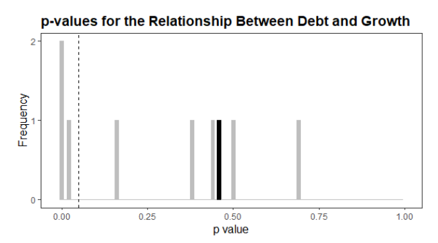
Thus, researchers can choose from a bunch of reasonable combinations of control variables. Does this affect the outcomes? To test this, we ran multiple analyses about the relationship between general government debt and growth rates across a sample of countries worldwide.³ Working with a set of nine widely used control variables,⁴ we ran one analysis with all control variables, and nine additional analyses where we removed one of the controls. The distribution of the p-values is displayed below. 

First, the black bar shows the p-value for the analysis using the complete set of control variables. Here, the relationship between debt and growth rates was insignificant (p = .458). Yet, when removing one of the nine control variables, the results can change drastically, as demonstrated by the grey bars: Two analyses (one without life expectancy and the other without inflation rates) found that higher debt levels were highly significantly associated with lower growth, with p-values of .003 and < .001, respectively. Additionally, another analysis (this time without investment levels) detected a significant negative relationship, too, p = .023.⁵ All remaining analyses were, however, not even close to being significant. 

Why do p-values change when we include or exclude different control variables? Generally, there are two main reasons for this: 

• Control variables might reduce noise in the outcome variable: By including control variables, we might explain some of the variation in the outcome (here: growth rates). This reduces the "noise" in its values, so it is easier to detect the effect of the predictor of interest (here: debt). 

• They might, however, also account for relationships between variables: Control variables may be related to both the predictor of interest and the outcome. By including these controls, we isolate the unique contribution of debt to growth rates. Without them, we might mistakenly attribute some of the control variable's effect to debt. 

The second case is particularly interesting because it changes how we (should) interpret the regression results. For example, if we do not control for inflation rates, the observed relationship between debt and growth might not be due to debt itself reducing growth. Instead, it could reflect the fact that higher debt levels are often associated with high inflation, which in turn hampers growth. In this case, failing to control for inflation could lead us to a misleading conclusion about the causal relationship between debt and growth. However, not many papers reporting growth regressions seem to discuss how their composition of control variables affects the outcomes; instead, it appears more common to choose a particular set based on previous research (e.g., a popular paper by Barro, 1991) that might be more or less appropriate for different regressions. 

This quick example demonstrates that the set of control variables heavily influences whether a predictor for economic growth will be significant or not.⁶ It also shows that, given the lack of consensus about which variables to control for, researchers have a fair chance of generating positive results by playing with the controls. 

Year 
Another standard research design in cliometrics or cultural research is the cross-section, where we score countries on a predictor and then examine whether this predictor is significantly related to an outcome: Does an individualistic (vs. collectivistic) culture relate to higher productivity (Gorodnichenko & Roland, 2017)? Do countries with low, medium, or high genetic diversity have a higher GDP per capita (Q. Ashraf & O. Galor, 2013)? For such comparisons, we must select a reference year—does an individualistic culture relate to higher productivity in 2000, 2010, or 2020? 

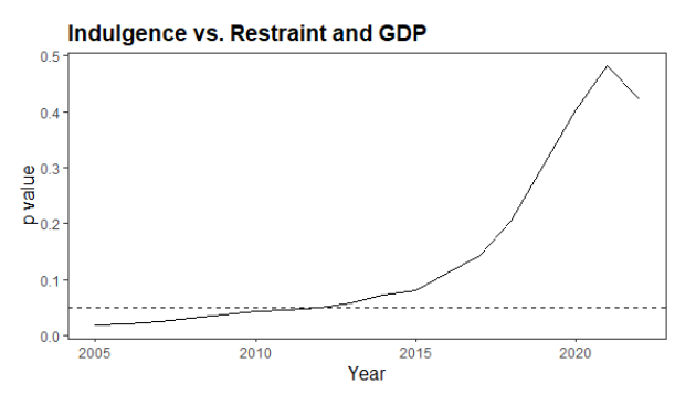
To demonstrate that the year matters, we set up a quick example analysis: Is indulgence vs. restraint (i.e., the degree to which relatively free gratification of basic human needs is restricted by, for instance, social norms; Hofstede, 1980) associated with GDP per capita?⁷ The graphic below shows the p values for the years between 2005 and 2022: 

First, the analyses for all years indicate that indulgence is positively related to GDP per capita. However, while this relationship is significant for the years between 2005 and 2012 (and marginally significant until 2015), it becomes insignificant afterward. This could be due to some short-term developments: for example, some very restrained countries (e.g., China and Pakistan) experienced relatively high growth rates during our investigation period, while some very indulgent countries (e.g., Argentina and Brazil) struggled more. Still, it could also reflect that the relationship between indulgence/restraint and economic performance became weaker over time. In any case, the common practice of picking one year seems misplaced for this particular analysis, as developments characteristic of that year but not of the research question of interest could determine whether we observe a (significant) relationship or not. Instead, it might be more appropriate to look at the development of the relationship over time: accounting for variation between the results of different years might not only prevent false positives (or negatives) but also detect long-term developments in a relationship that could, in turn, be exploited for theory-building (e.g., Maseland, 2021). 

The analyses reveal a consistent positive relationship between indulgence and GDP per capita across all years. However, this relationship is significant only between 2005 and 2012 (and marginally significant until 2015) but becomes insignificant in later years. This shift could reflect short-term developments during the study period: for instance, some highly restrained countries, like China and Pakistan, experienced relatively high economic growth, while the economies of more indulgent countries, such as Argentina and Brazil, struggled at the start of the millennium. Alternatively, the fluctuations might also indicate that the relationship between indulgence/restraint and economic performance has weakened over time. 

In either case, relying on data from a single year seems problematic for this kind of analysis. A snapshot from one year could be heavily influenced by events specific to that period that determine the answer we receive to our broader research question. It would be more meaningful to examine how this relationship evolves over time. By considering variations across multiple years, researchers can not only reduce the risk of false positives (or negatives) but also uncover long-term trends that might inform theory development (see, e.g., Maseland, 2021). Such an approach could help identify persistent patterns or shifts in the relationship, providing valuable insights into the dynamics between cultural traits and economic performance. 

Conclusion 
This blog post aimed to establish two fundamental notions: First, quantitative analysis in the arts (e.g., history, cultural research) also involves researcher degrees of freedom, which can lead to meaningful variations in results. Second, these degrees of freedom can be strategically utilized to generate significant findings. 

Together, these two notions could lead to an inflated number of false-positive results. Indeed, the limited evidence we have so far suggests the existence of at least some publication bias and/or selective reporting in the quantitative humanities. Finally, while research in the humanities may not share the same topics or degrees of freedom as fields like psychology or medicine, the approaches that meta-researchers have developed in recent years (e.g., multiverse analyses, p-curves) could provide a good starting position for addressing publication bias and selective reporting in the arts as well. 

References 

Acemoglu, D., Johnson, S., & Robinson, J. (2005). The Rise of Europe: Atlantic Trade, Institutional Change, and Economic Growth. American Economic Review, 95(3), 546-579. https://doi.org/10.1257/0002828054201305  

Acemoglu, D., Johnson, S., & Robinson, J. A. (2012). The Colonial Origins of Comparative Development: An Empirical Investigation: Reply. American Economic Review, 102(6), 3077-3110. https://doi.org/10.1257/aer.102.6.3077  

Albouy, D. Y. (2012). The Colonial Origins of Comparative Development: An Empirical Investigation: Comment. American Economic Review, 102(6), 3059-3076. https://doi.org/10.1257/aer.102.6.3059  

Angelucci, C., Meraglia, S., & Voigtländer, N. (2022). How Merchant Towns Shaped Parliaments: From the Norman Conquest of England to the Great Reform Act. American Economic Review, 112(10), 3441-3487. https://doi.org/10.1257/aer.20200885  

Ashraf, Q., & Galor, O. (2013). The “Out of Africa” Hypothesis, Human Genetic Diversity, and Comparative Economic Development. American Economic Review, 103(1), 1-46. https://doi.org/10.1257/aer.103.1.1  

Astington, J. W. (1999). The language of intention: Three ways of doing it. In P. D. Zelazo, J. W. Astington, & D. R. Olson (Eds.), Developing theories of intention. Erlbaum.  

Bargh, J. A., Chen, M., & Burrows, L. (1996). Automaticity of social behavior: Direct effects of trait construct and stereotype activation on action. Journal of Personality and Social Psychology, 71(2), 230-244. https://doi.org/10.1037/0022-3514.71.2.230  

Barro, R. J. (1991). Economic growth in a cross section of countries. The Quarterly Journal of Economics, 106(2), 407. https://doi.org/10.2307/2937943 

Berger, D., Easterly, W., Nunn, N., & Satyanath, S. (2013). Commercial Imperialism? Political Influence and Trade During the Cold War. American Economic Review, 103(2), 863-896. https://doi.org/10.1257/aer.103.2.863  

Berggren, N., Bergh, A., & BjØRnskov, C. (2011). The growth effects of institutional instability. Journal of Institutional Economics, 8(2), 187-224. https://doi.org/10.1017/s1744137411000488  

Bratman, M. E. (1987). Intention, plans, and practical reason. MIT Press.  

Campbell, D., Brodeur, A., Dreber, A., Johannesson, M., Kopecky, J., Lusher, L., & Tsoy, N. (2024). The Robustness Reproducibility of the American Economic Review (124). https://www.econstor.eu/bitstream/10419/295222/1/I4R-DP124.pdf 

Cova, F., Strickland, B., Abatista, A., Allard, A., Andow, J., Attie, M., Beebe, J., Berniūnas, R., Boudesseul, J., Colombo, M., Cushman, F., Diaz, R., N’Djaye Nikolai van Dongen, N., Dranseika, V., Earp, B. D., Torres, A. G., Hannikainen, I., Hernández-Conde, J. V., Hu, W.,…Zhou, X. (2018). Estimating the Reproducibility of Experimental Philosophy. Review of Philosophy and Psychology, 12(1), 9-44. https://doi.org/10.1007/s13164-018-0400-9  

De Rijcke, S., & Penders, B. (2018). Resist calls for replicability in the humanities. Nature, 560(7716), 29. https://doi.org/10.1038/d41586-018-05845-z 

Gorodnichenko, Y., & Roland, G. (2017). Culture, Institutions, and the Wealth of Nations. The Review of Economics and Statistics, 99(3), 402-416. https://doi.org/10.1162/REST_a_00599  

Guinnane, T. W., & Hoffman, P. (2022). Medieval Anti-Semitism, Weimar Social Capital, and the Rise of the Nazi Party: A Reconsideration. SSRN Electronic Journal. https://doi.org/10.2139/ssrn.4286968  

Hofstede, G. (1980). Culture's Consequences: International Differences in Work-Related Values. Sage Publications.  

Knobe, J. (2003). Intentional action in folk psychology: An experimental investigation. Philosophical Psychology, 16(2), 309-324. https://doi.org/10.1080/09515080307771  

Latour, B. (1991). We have never been modern. Harvard University Press.  

Maseland, R. (2021). Contingent determinants. Journal of Development Economics, 151. https://doi.org/10.1016/j.jdeveco.2021.102654  

Nelson, L. D., Simmons, J., & Simonsohn, U. (2018). Psychology&apos;s Renaissance. Annual Review of Psychology, 69(Volume 69, 2018), 511-534. https://doi.org/https://doi.org/10.1146/annurev-psych-122216-011836  

Open Science Collaboration. (2015). PSYCHOLOGY. Estimating the reproducibility of psychological science. Science, 349(6251), aac4716. https://doi.org/10.1126/science.aac4716  

Peels, R., Van Den Brink, G., Van Eyghen, H., & Pear, R. (2024). Introduction: Replicating John Hedley Brooke’s work on the history of science and religion. Zygon, 59(2). https://doi.org/10.16995/zygon.11255 

Rennie, D., & Flanagin, A. (2018). Three Decades of Peer Review Congresses. JAMA, 319(4), 350-353. https://doi.org/10.1001/jama.2017.20606  

Voigtländer, N., & Voth, H.-J. (2022). Response to Guinnane and Hoffman: Medieval Anti-Semitism, Weimar Social Capital, and the Rise of the Nazi Party: A Reconsideration. SSRN Electronic Journal. https://doi.org/10.2139/ssrn.4316007  

Wicherts, J. M., Veldkamp, C. L., Augusteijn, H. E., Bakker, M., van Aert, R. C., & van Assen, M. A. (2016). Degrees of Freedom in Planning, Running, Analyzing, and Reporting Psychological Studies: A Checklist to Avoid p-Hacking. Front Psychol, 7, 1832. https://doi.org/10.3389/fpsyg.2016.01832  

Footnotes
1. For example, the theory of unconscious priming was originally corroborated by verifying the hypothesis ‘‘People walk slower when they are shown words they associate with the elderly” (Bargh et al., 1996). Compared to that, it is very hard to establish (inter-subjective) falsification of, say, the central hypothesis of Bruno Latour’s We Have Never Been Modern (Latour, 1991) “What we call the modern world is based on an ill-defined separation between nature and society.” 

2. Also, an interesting account by de Rijcke and Penders (2018 suggests that the arts are more about the search for meaning than chasing after truth and perform “evaluation and assessment according to different quality criteria — namely, those that are based on cultural relationships and not statistical realities.” In this case, the problem of overconfidence in or flaws of the theoretical state of the art(s) is irrelevant and any efforts to detect such issues redundant. Still, as Peels et al. (2024) note, the arts are not entirely off the hook when it comes to truth-seeking, as they also include research questions such as whether European colonies that were poorer at the end of the Middle Ages developed better than richer colonies because they were not subject to extractive institutions (Acemoglu et al., 2002). Therefore, this blog post at least concerns questions of this type, without explicitly including or excluding any other research question from the arts. 

3. Growth rates were calculated using the data from the Maddison Project Database 2023 (Bolt & van Zanden, 2023). Data about general government debt came from the Global Debt Database of the International Monetary Fund (Mbaye et al., 2018). The sources of the control variables were the Penn World Tables 10.01 (Feenstra et al., 2015), the World Development Indicators (World Bank, 2024), ILOSTAT (International Labour Organization, 2024), and Barro and Lee (2013). We used data from 2005 to 2019. 

4. The control variables were GDP capita (for convergence), population growth, investment levels relative to the GDP, government share relative to the GDP, sum of imports and exports relative to the GDP, education level, inflation level, life expectancy, and labor force growth. 

5. The coefficients indicate that a 25% increase in general government debt (similar to the increase in the United States during the first year of the COVID-19 pandemic) decreases yearly growth rates by 0.3% to 0.4%. 

6. Interestingly, the effect size estimates are rather close to one another, ranging from 0.0% to 0.4% for all (significant and insignificant) analyses. The underlying multiverse variability is 0.014 for Cohen’s f².  

7. GDP data came from the Maddison Project Database 2023 (Bolt & van Zanden, 2023), and data for power distance from the Hofstede (1980) data. We performed a linear regression for each year, controlling for a standard set of geographical and religious variables already used by previous studies on the relationship between culture and economic performance (e.g., Gorodnichenko & Roland, 2017).